── Attaching core tidyverse packages ──────────────────────── tidyverse 2.0.0 ──
✔ dplyr     1.1.4     ✔ readr     2.1.5
✔ forcats   1.0.0     ✔ stringr   1.5.1
✔ ggplot2   3.4.4     ✔ tibble    3.2.1
✔ lubridate 1.9.3     ✔ tidyr     1.3.1
✔ purrr     1.0.2
── Conflicts ────────────────────────────────────────── tidyverse_conflicts() ──
✖ dplyr::filter() masks stats::filter()
✖ dplyr::lag()    masks stats::lag()
ℹ Use the conflicted package (<http://conflicted.r-lib.org/>) to force all conflicts to become errors
Merging VCF Files
The first thing we need to to is zip and then index the individual vcf files. As a reminder, these files have been created by individual freebayes SNP calling of chunks of individuals partitioned into groups based upon the first letter of the popualtion from which they were collected. So, in the following examples, the file R.vcf contains all the individuals in populations starting with the letter R. When there are not that many individuals in a group, they are clustered—below we have JK.vcf which has all the individuals from populations starting with the letters J and K.
So, lets compress these raw files first.
% bgzip JK.vcf
% bgzip P.vcf
% bgzip R.vcf
% bgzip S.vcf
% bgzip W.vcf
% ls -alh
total 70032
drwxr-xr-x   7 rodney  staff   224B Feb 16 14:22 .
drwxr-xr-x  21 rodney  staff   672B Feb 16 14:10 ..
-rw-r--r--   1 rodney  staff   3.1M Feb 16 14:20 JK.vcf.gz
-rw-r--r--   1 rodney  staff   5.8M Feb 16 14:22 P.vcf.gz
-rw-r--r--   1 rodney  staff   4.6M Feb 16 14:22 R.vcf.gz
-rw-r--r--   1 rodney  staff    14M Feb 16 14:22 S.vcf.gz
-rw-r--r--   1 rodney  staff   5.8M Feb 16 14:22 W.vcf.gz
Now we need to index these files.
% tabix -p vcf JK.vcf.gz
% tabix -p vcf P.vcf.gz
% tabix -p vcf R.vcf.gz
% tabix -p vcf S.vcf.gz
% tabix -p vcf W.vcf.gz
Then we can merge the files together into a single file. Here, the output file indicates the populations that contribute to it.
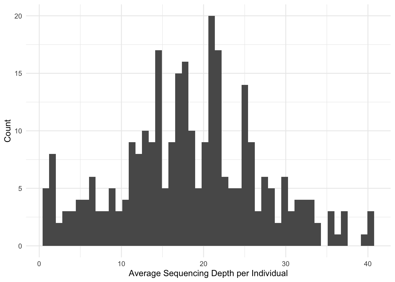
% vcf-merge JK.vcf.gz P.vcf.gz R.vcf.gz S.vcf.gz W.vcf.gz > JKPRSW.vcfSo here are a few things that I’ve found that provide some insights into the data we are getting. Here is the sequencing depth per individual for only the SNP sites who have a minimum quality score of 20.
% vcftools --vcf JKPRSW.vcf --remove-indels --minQ 20 --depth -c > depth.txtThis produced a distribution of sequencing depths for these individuals.
Alternatively—and perhaps more important for us—we can look at the per-site depths. The goal here is to retain sites that have enough sequencing depth such that we are confident that it is a good site but not too much such that it is a reapeaty region in the geniome. For simplicity, I’ll drop the lower and upper standard deviation.
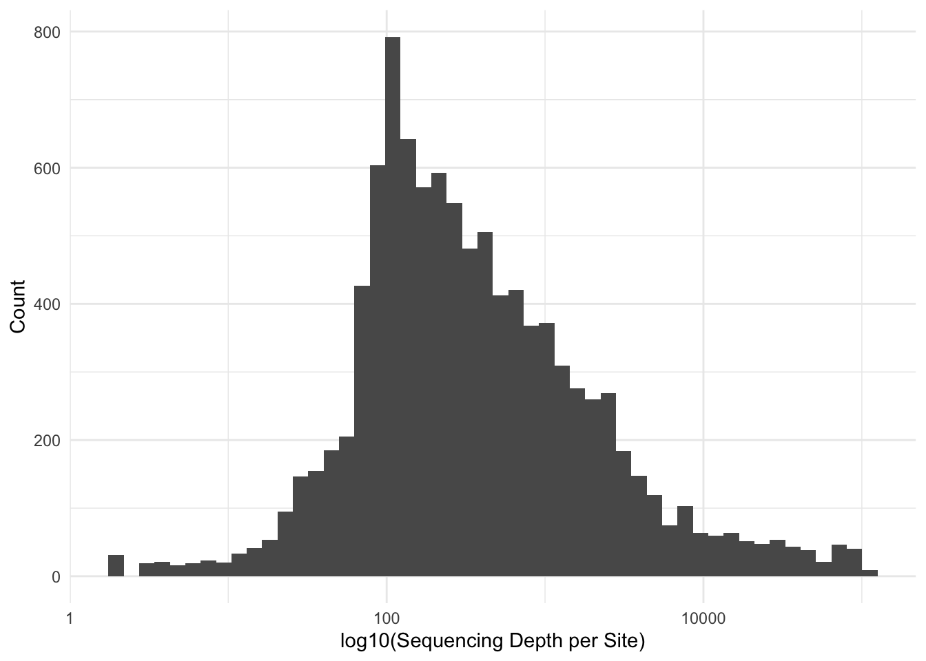
For simplicity, I’m just going to take the inner-50% of the data, dropping off the lower and upper quantiles.
quantile( site_depth$SUM_DEPTH,
          prob = c(0.10,0.25, 0.5, 0.75, 0.90))
10% 25% 50% 75% 90%
60.0 110.0 278.0 964.0 3421.1 This leaves us with 5047 sites.
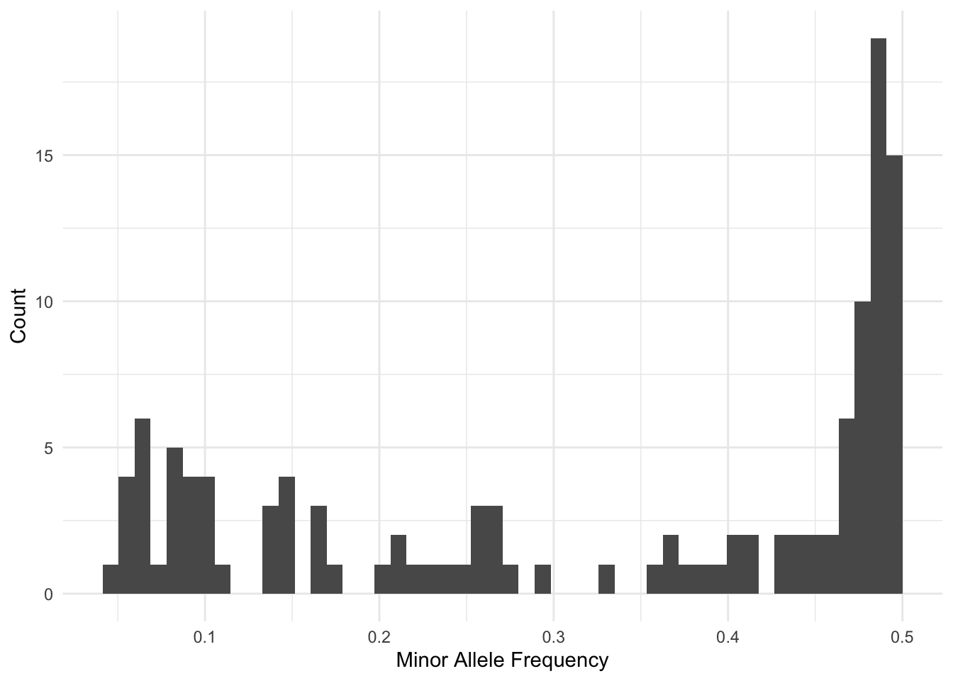
Now, we can go back to vcftools and use these values to select only sites with a quality score exceeding 20, and are in the middle 50 percentile of the depth coverage and have a minor allele frequency of at least 5%.
% vcftools --vcf JKPRSW.vcf --remove-indels --min-meanDP 110 --max-meanDP 964 --minQ 20 --maf 0.05  --min-alleles 2 --max-alleles 2 --freq
After filtering, kept 302 out of 302 Individuals
Outputting Frequency Statistics...
After filtering, kept 120 out of a possible 22604 Sites
Run Time = 1.00 seconds
So, we have 120 loci to work with from this subset.
Filtering out Sequncing Errors
Now, I’m going to look at the effects of filter different aspects. Here is the minor allele count (MAC). I’m doing this over frequency given that I have \(N=1419\) individuals.
tribble( ~MAC, ~SNPs,
         2,  934,
         5,  843,
         10, 745,
         25, 568,
         50, 386,
         75, 294,
         100, 223,
         150, 155,
         200, 90) %>%
  mutate( p = MAC/(2*1419)) %>%
  ggplot( aes(MAC, SNPs) ) +
  geom_line() +
  geom_point() +
  xlab("Minor Allele Count") +
  ylab("SNP Loci Identified")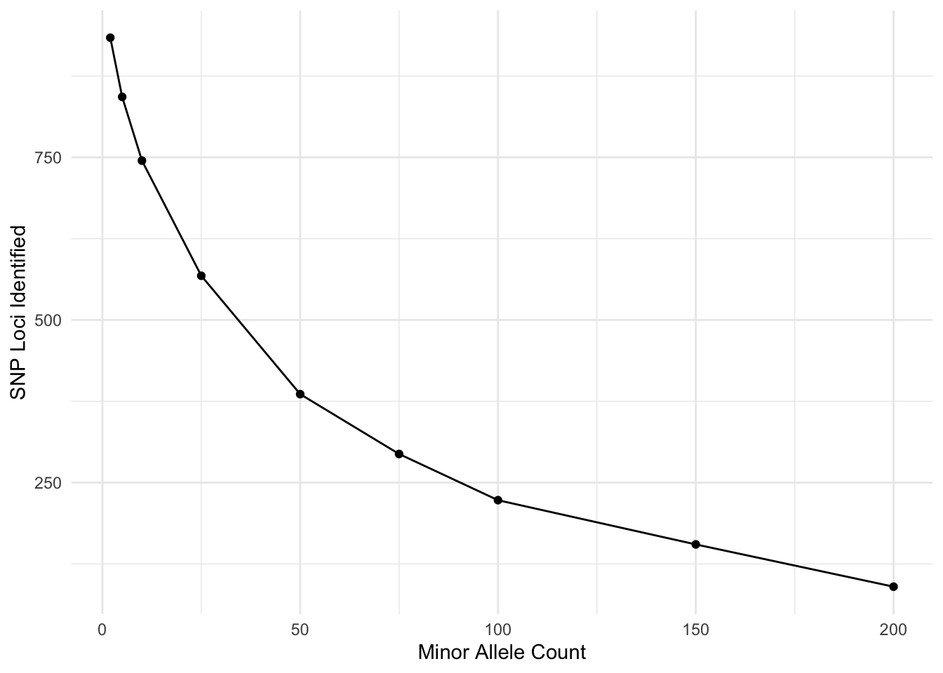
I am sure there is a probability example that could be used here to look at where you break even on sequencing errors and joint probability of the same allele being incorrectly identified. Don’t quite want to work it out right now but I think my 5% (putting it just shy of the MAC=150) may have been a bit too stringent…
Filtering on Depth
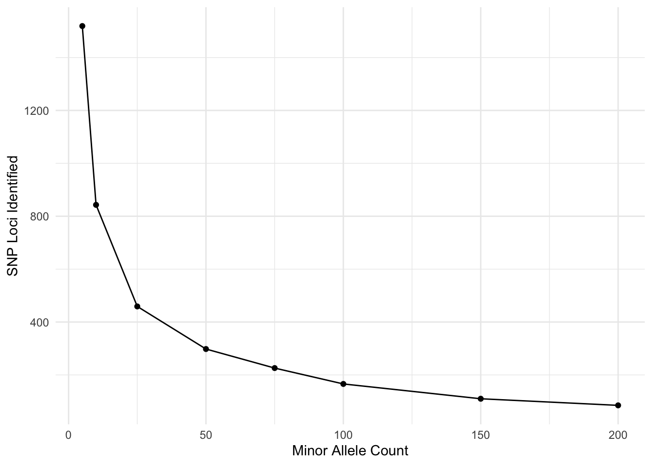
Next lets look at sequencing depth. Here i am going to fix the MAC=5 and cut off all the loci that have a depths in excess of the 90% in depths (see above) and then look at how many loci are recovered going from 5X coverage up to 200X (the example above had it set at a minimum coverage of 110X).
tribble( ~`Minimum Depth`, ~SNPs,
         5,  1519,
         10, 843,
         25, 459,
         50, 298,
         75, 226,
         100, 166,
         150, 110,
         200, 85) %>%
  ggplot( aes(`Minimum Depth`, SNPs) ) +
  geom_line() +
  geom_point() +
  xlab("Minor Allele Count") +
  ylab("SNP Loci Identified")