library( raster )
url <- "https://github.com/dyerlab/ENVS-Lectures/raw/master/data/alt_22.tif"
raster( url ) %>%
  crop(extent( -111.6, -111, 25.6, 26.2) ) -> baja_california
plot( baja_california ) 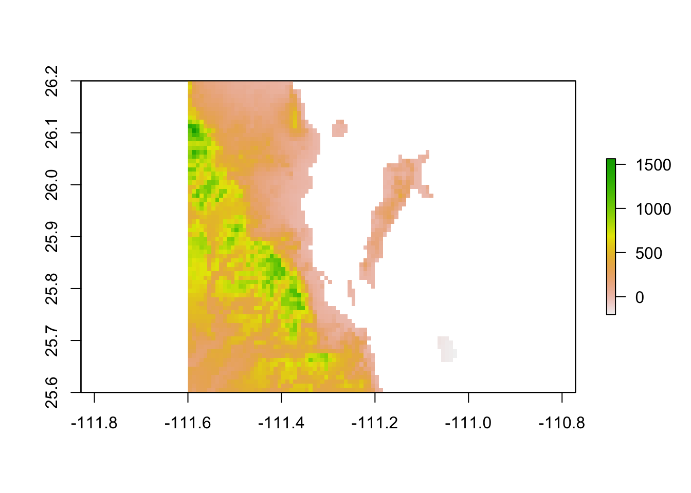
So let’s load in a raster and crop it down to look at it. Here is the area surrounding Loreto, BCS Mexico as represented by a 1-km resolution raster of elevation.
library( raster )
url <- "https://github.com/dyerlab/ENVS-Lectures/raw/master/data/alt_22.tif"
raster( url ) %>%
crop(extent( -111.6, -111, 25.6, 26.2) ) -> baja_california
plot( baja_california )
For simple viewing, we can tell the plot to interpolate it, which will shape it a bit. This does not change the data, it only shows the data a bit differently.
plot( baja_california, interpolate = TRUE )
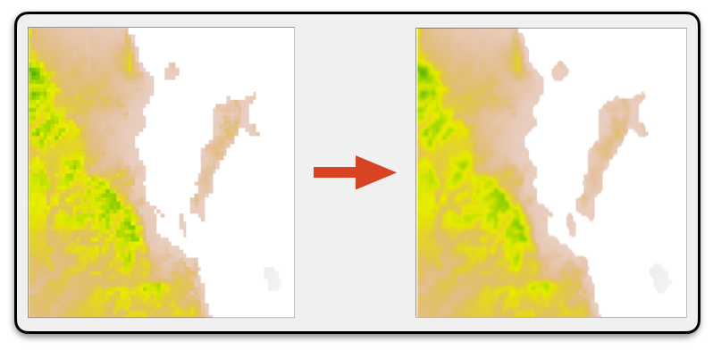
We can also resample the data, which changes it. We can disaggregate it, which makes a new raster with a more fine grain resolution and interpolates the new values to fit.
loreto_disaggregated <- disaggregate( baja_california,
                                      fact = 5,
                                      method = "bilinear")
which takes the previous raster whose size was:
dim( baja_california )[1] 72 72 1and makes the new one of size
dim( loreto_disaggregated )[1] 360 360 1as the fact=5 means that each cell in baja_california is turned into a 5x5 set of cells whose values are interpolated. Notice in the plot below, how the pixelation is reduced around the coast (this raster has all water = NA).
plot( loreto_disaggregated )
We can also smooth it using a custom focal operation based upon a matrix of values and a function we define for it. Here the weight (w) matrix is a 5x5 matrix of 1 (defining the values around each spot that will be used) and the fun=mean will take the average of the 5x5 matrix of values.
loreto_focal <- focal( baja_california,
                       w = matrix(1, 5, 5),
                       fun = mean,
                       na.rm=TRUE)
This approach does not change the resoution of each cell, it only smooths it out. I also ignored NA for those edge cases.
dim( loreto_focal )[1] 72 72 1And if you look at it, it still has some pixelation (minecraft-i-ness if you will)
plot( loreto_focal )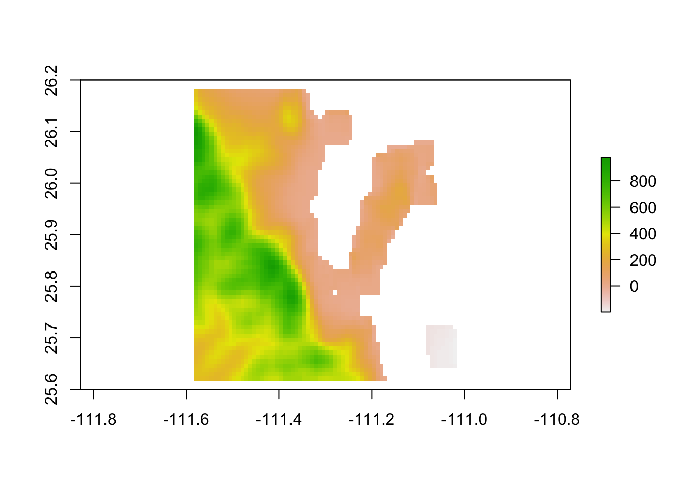
The method you choose is up to you and the consequences of changing the raw data. Be careful.